Introduction¶

forgi.threedee is an extension of forgi capable of handling 3D data about RNA structures. It provides methods for extracting secondary structure as well as creating a coarse grain representation of 3D RNA structures.

Requirements¶

We strongly recommend installing MC_Annotate or DSSR when using forgi to work with PDB files. See Optional, external dependencies (require manual installation)

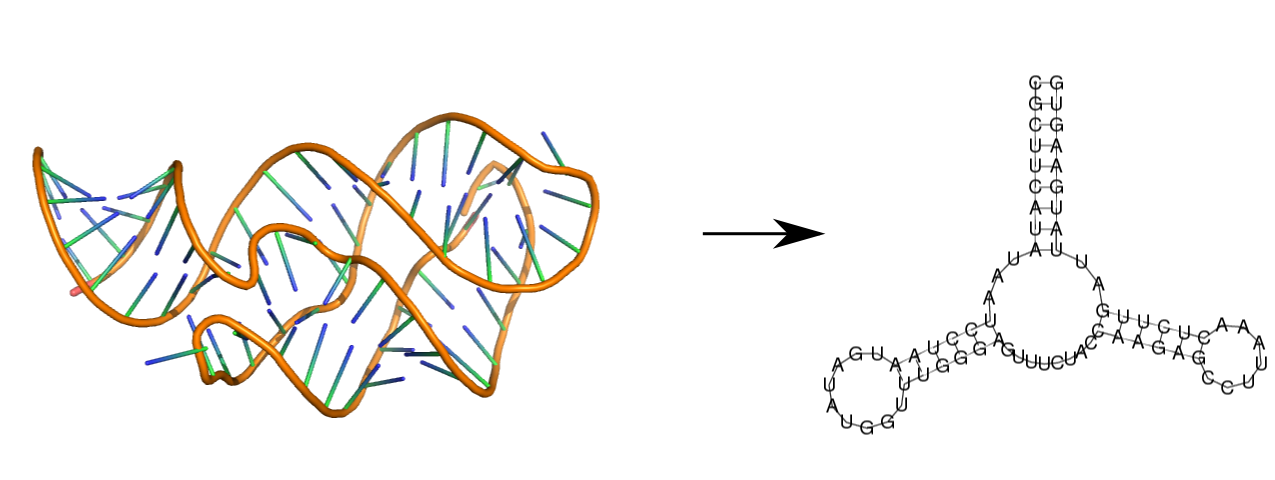
Extracting 2D structure from a 3D structure¶

To extract the base-pair information from a 3D structure stored in a PDB or MMCIF file, just convert the file to a fasta file using the rnaConvert.py script:

$ rnaConvert.py -T fasta examples/1y26.pdb
>1y26
CGCUUCAUAUAAUCCUAAUGAUAUGGUUUGGGAGUUUCUACCAAGAGCCUUAAACUCUUGAUUAUGAAGUG
(((((((((...(((((((.......)))))))........((((((.......))))))..)))))))))

This can also be done programmatically in python:

>>> cg, = forgi.load_rna('test/forgi/threedee/data/1y26.pdb')
>>> print( cg.to_fasta_string() )
>1y26_X
CGCUUCAUAUAAUCCUAAUGAUAUGGUUUGGGAGUUUCUACCAAGAGCCUUAAACUCUUGAUUAUGAAGUG
((((((((((..((((((.........))))))......).((((((.......))))))..)))))))))

Pseudoknots are removed using the knotted2nested.py script which is included with the generous permition of Dr. Sandra Smit [1]. Users making use of this feature of the 3D-to-2D facilities of the forgi.threedee package should cite the articles listed in the citations section at the bottom of this page.

To keep pseudoknots, use the --pseudoknots commandline option to rnaConvert.py or pdb_remove_pk=False in the load_rna function.

Creating a Coarse Grain 3D Representation of an RNA Molecule¶

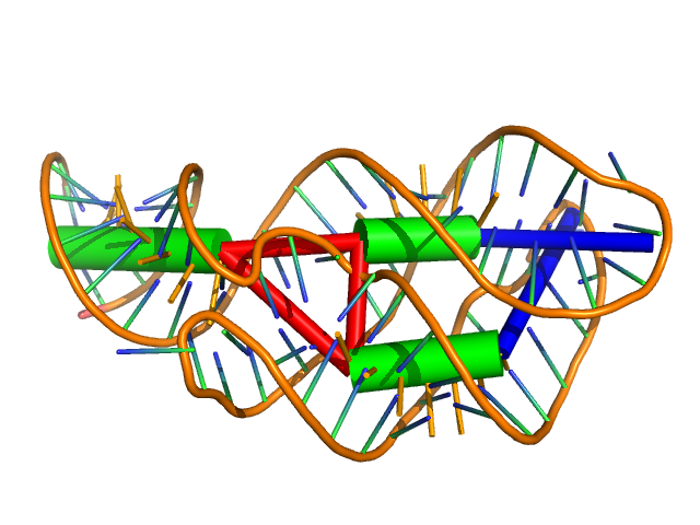
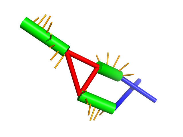
One can imagine an RNA molecule as a collection of helices and … not helices (hairpins, interior loops, multiloops, etc..) as described in the RNA Secondary Structure as a Graph Using the forgi Library. By creating an abstraction for the canonical helixes and representing them as cylinders, we can create a coarse grain representaiton of the RNA molecule:

$ python rnaConvert.py -T forgi 2l94.pdb
name 2l94_A
length 45
seq GGGAAGAUCUGGCCUUCCCACAAGGGAAGGCCAGGGAAUCUUCCC
seq_ids A:1 A:2 A:3 A:4 A:5 A:6 A:7 A:8 A:9 A:10 A:11 A:12 A:13 A:14 A:15 A:16 A:17 A:18 A:19 A:20 A:21 A:22 A:23 A:24 A:25 A:26 A:27 A:28 A:29 A:30 A:31 A:32 A:33 A:34 A:35 A:36 A:37 A:38 A:39 A:40 A:41 A:42 A:43 A:44 A:45
define s0 1 8 38 45
define i0 35 37
define s1 9 19 24 34
define h0 20 23
connect s0 i0
connect s1 i0 h0
coord s1 -3.1866813709154620 3.4914107521504016 3.6351776728651553 21.4829112410527117 -2.1083990492427773 0.5057319475413644
coord s0 -25.6897073719667972 -5.8096386325483751 -4.0265189300856425 -10.6552743590351255 3.1029175167846290 -0.4045073529842251
coord h0 21.4829112410527117 -2.1083990492427773 0.5057319475413644 29.0380001068115234 4.4409999847412109 -5.3439998626708984
twist s1 -0.0184282079893236 0.4246648355404593 -0.9051630674114455 -0.1571049415641848 -0.1462958719913227 -0.9766860064393329
twist s0 -0.5333577254411702 0.8264653710187239 0.1802346448913319 0.4343359029793392 -0.4058832531020076 -0.8041213268123496
interacting A:28
interacting A:17
interacting A:11
interacting A:16
interacting A:10
interacting A:15
interacting A:9
interacting A:14
interacting A:34
interacting A:12
interacting A:33
interacting A:27
interacting A:32
interacting A:26
interacting A:31
interacting A:25
interacting A:30
interacting A:29
vres i0 -2.31427602 1.57444474 3.54455842 -7.71669904 4.28261433 4.39684139 -5.20558252 8.97808845 5.88005184
vres h0 -2.11144177 4.89881497 -3.76862411 0.26981184 0.20644734 -4.70205156 5.79209284 -0.00000000 0.00000000 3.79477715 2.83408417 3.24575331

The file format is an extention of the BulgeGraph file format (The forgi fileformat for secondary structure). The lines beginning with coord indicate the positions of the helices. They are calculated by fitting a cylinder to each helical region of the 3D structure.

The seq_ids line is used to store the residue numbers used in the PDB prefixed by the chain (For more on residue numbering see …). The interacting lines give residues that interact with a non-RNA molecule, in this case a ligand. The vres lines give the positions of the C1’ atom of the residues in loops (Always 3 coordinates correspond to one residue). If the C1’ atom is missing, the coordinates refer to a very approximate position instead.

Visualizing the Coarse Grain Helical Representation¶

The coarse grain representation shown in the prior example can be visualized using Pymol and the visualize_rna.py script. The green cylinders below represent canonical helical regions, red represent multiloops and blue - hairpin loops:

visualize_rna.py 1y26.pdb

The visualize_rna.py script can also display files in the forgi file format:

visualize_rna.py examples/1y26.cg

Calculate the Distance Between Two Coarse-Grain Elements¶

>>> cg, forgi.load_rna('test/forgi/threedee/data/1y26.cg')
>>> dist = cg.element_physical_distance('h0', 'h1')
>>> print (dist)
7.87989954482

Find out How Much an Interior Loop Bends a Stem¶

Interior loops often place kinks in long stem-like structures. This leads to a change in the base stacking pattern and can indicate functional relevance. To extract this information for a given PDB file, we need to iterate over each interior loop and calculate the angle between the two stems it connects:

>>> import forgi.threedee.utilities.vector as ftuv
>>> cg = forgi.load_rna('test/forgi/threedee/data/1GID_native.pdb')
>>> for iloop in cg.iloop_iterator():
...     conn = cg.connections(iloop)
...     # conn contains two values ['s0', 's1']
...     angle = ftuv.vec_angle(cg.coords.get_direction(conn[0]), cg.coords.get_direction(conn[1]))
...     print(iloop, angle)
...
i3 0.307770762476
i2 2.74681004918
i1 0.1697963999
i0 0.491755788011
i5 0.456253974086
i4 0.261428615896
i7 0.15810445353
i6 0.510919193909

conn[0] and conn[1] are the identifiers of the first and second connected stems, respectively. cg.coords[conn[0]][0] contains the coordinates of the front end of the first stem and cg.coords[conn[0]][1] the end coordinates. cg.coords.get_direction(conn[0]) gives the vector from the stem start to the stem end, i.e. cg.coords[conn[0]][1] -  `cg.coords[conn[0]][0]. We then use these direction vectors to calculate the angle in radians. This example, using the Group-I intron, indicates the presence of a kink-turn at interior loop i2.

Check if a Bio.PDB Chain is RNA¶

Example:

>>> import Bio
>>> import forgi.threedee.utilities.pdb as ftup
>>> import os.path as op
>>>
>>> filename = op.expanduser('~/data/pdbs/1Y26.pdb')
>>> structure = Bio.PDB.PDBParser().get_structure('blah', filename)
>>> ftup.is_rna(list(structure.get_chains())[0])
True

Calculate the RMSD Between two PDB Chains¶

The root mean square deviation (RMSD) is a measure of how much two molecules differ in their atomic coordinates. The value, of course, depends on how the two molecules are superimposed, but in most cases (including here) a rotation and translation is applied such that the RMSD is minimized. The RMSD value is often used to compare the models created by structure prediction software to the real structure, and can easily be calculated using the pdb_rmsd method. It can take an optional sidechains parameter (which defaults to False), to indicate that the sidechains (bases) should be included in the RMSD calculation. If it is False, then only the backbone atoms are used in the calculation:

>>> import forgi.threedee.utilities.pdb as ftup
>>> import Bio.PDB as bpdb
>>> c = list(bpdb.PDBParser().get_structure('temp', 'test/forgi/threedee/data/2mis.pdb').get_chains())[0]
>>> ftup.pdb_rmsd(c, c)
(180, 1.0314194769216807e-14, (array([[  1.00000000e+00,  -1.94289029e-16,   1.11022302e-16],
       [  8.32667268e-17,   1.00000000e+00,   6.93889390e-17],
              [ -5.55111512e-17,   6.93889390e-17,   1.00000000e+00]]), array([ -5.68434189e-14,   2.84217094e-14,  -1.73194792e-14])))

The return value is a tuple containing the number of atoms that were superimposed, the RMSD value and another tuple containing the optimal rotation matrix and translation vector.

This can also be achieved using the compareRNA.py script:

$ compare_RNA.py 'test/forgi/threedee/data/2mis.pdb' 'test/forgi/threedee/data/2mis.pdb' --pdb-rmsd
PDB-RMSD (chains A):        0.000

Calculate the RMSD Between two Coarse-Grain Models¶

Like PDB chains, we can also compute an RMSD value for two coarse grain models. For this we need to use the virtual residues of the helices as the atoms and compute the RMSD value amongst them:

>>> import forgi.threedee.model.coarse_grain as ftmc
>>> import forgi.threedee.model.similarity as ftms
>>>
>>> cg1, = forgi.load_rna('test/forgi/threedee/data/1y26.cg')
>>> cg2, = forgi.load_rna('test/forgi/threedee/data/1y26.cg')
>>>
>>> print ftms.cg_rmsd(cg1,cg2)
0.0

If we like more control, we can export any list of coordinates from the coarse grain moidel that is in a defined order and calculate the rmsd between these two point clouds. Examples would include the start and end coordinates of every stem for a faster RMSD estimation that is less accurate but avoids the overhead of generating the virtual residues.

Note that currently forgi.threedee.model.similarity.rmsd centers and optimallly rotates the two point clouds to minimize the RMSD. For an uncentered RMSD use forgi.threedee.utilities.vector.vector_set_rmsd

>>> import forgi.threedee.model.coarse_grain as ftmc
>>> import forgi.threedee.utilities.graph_pdb as ftug
>>> import forgi.threedee.model.similarity as ftms
>>>
>>> cg1, = forgi.load_rna('test/forgi/threedee/data/1y26.cg')
>>> cg2, = forgi.load_rna('test/forgi/threedee/data/1y26.cg')
>>>
>>> coords1 = cg1.get_ordered_stem_poss()
>>> coords2 = cg2.get_ordered_stem_poss()
>>>
>>> print ftms.rmsd(coords1, coords2)
0.0

Scalar descriptors of RNA 3D structures¶

To characterize an RNA 3D structures, a lot of descriptors could be potentially useful. The forgi.threedee.model.descriptors library includes the following scalar descriptors.

1. The Radius of gyration
2. The anisotropy
3. The asphericity

Note that 1-3 are related, as they could all be derived from the gyration tensor. An overview over these properties can be found for example in the introduction of reference [2] and in the papers referenced therein.

>>> import forgi.threedee.model.coarse_grain as ftmc
>>> import forgi.threedee.model.descriptors as ftmd
>>>
>>> cg, = forgi.load_rna('test/forgi/threedee/data/1y26.cg')
>>>
>>> print( "Radius of Gyration", cg.radius_of_gyration() )
>>>
>>> coords = cg.get_ordered_stem_poss() #Use only coarse grained coordinates of stems
>>> coords = cg.get_ordered_virtual_residue_poss() #Alternatively use coordinates of virtual residues
>>>
>>> print "Anisotropy", ftmd.anisotropy(coords)
>>> print "Asphericity", ftmd.asphericity(coords)

Determine if two Atoms are Covalently Bonded¶

The difference between covalently bonded and unbonded atoms needs to be taken into account when calculating clash scores. Covalently bonded atoms can be closer to each other in a real structure than unbonded atoms. Based on the identity of the atoms and their parent nucleotides, the is_covalent function tries to determine the whether two atoms are covalently bonded (not taking into account the geometry, but only the atom names). This only works for unmodified nucleotides.

Example:

>>> import forgi.threedee.utilities.pdb as ftup
>>> c = ftup.get_biggest_chain('test/forgi/threedee/data/2mis.pdb')
>>> ftup.is_covalent([c[10]["C3'"], c[10]["C4'"]])
True
>>> ftup.is_covalent([c[10]["C3'"], c[10]["C5'"]])
False

Determine the total rotation of a stem¶

The location of a stem’s minor groove at the beginning and the end of the stem is stored as the twist vector. To calculate the total rotation of a stem, we need to calculate the angle between the two twist vectors and find out how many full turns around the helix we took.

An ideal helix turns 36.4 degrees per base-pair, so given the number of basepairs we can calculate the number of full turns.

Citations¶

[1] Sandra Smit, Kristian Rother, Jaap Heringa, and Rob Knight. From knotted to nested RNA structures: a variety of computational methods for pseudoknot removal. RNA (2008) 14(3):410-416.

[2] Handan Arkın and Wolfhard Janke. Gyration tensor based analysis of the shapes of polymer chains in an attractive spherical cage The Journal of Chemical Physics (2013) 138:054904, http://dx.doi.org/10.1063/1.4788616